
Quantum Principal Component Analysis (QPCA) is a hybrid dimensional-reduction algorithm that translates the covariance structure of classical data into a quantum density matrix and then employs Quantum Phase Estimation (QPE) to extract its eigenvalues. By simulating the unitary (where the density matrix is, QPCA can reveal the principal components of a data set while potentially leveraging quantum parallelism for speed-ups on large, high-dimensional data.
How Quantum PCA Differs from Classical PCA #
Classical PCA diagonalizes a covariance matrix on a classical computer, typically in time proportional to d features, returning eigenvectors and eigenvalues that quantify variance.
QPCA instead:
- Encodes the normalised covariance matrix as a quantum density matrix.
- Evolves that matrix under a simulated Hamiltonian to obtain a unitary operator.
- Applies Quantum Phase Estimation to recover phase angles proportional to the eigenvalues.
- Reconstructs principal-component variances from measured ancilla statistics.
The quantum-enhanced subroutines replace matrix diagonalisation with potentially poly-logarithmic depth circuits, shifting the computational bottleneck to state preparation and QPE rather than classical eigen decomposition.
How Quantum PCA Can Be Implemented #
- Data Normalisation and Preparation
- Convert raw numeric (or one-hot-encoded) data into a matrix X.
- Standardise each feature to zero mean and unit variance.
- Density-Matrix Construction
- Compute the classical covariance matrix
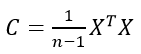
- Normalise to a valid density matrix

- Compute the classical covariance matrix
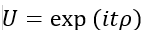
- Hamiltonian Simulation
- Exponentiate the density matrix:
- Pad to the nearest power-of-two dimension so that U acts on an integer number of qubits.
- Exponentiate the density matrix:
- Quantum Phase Estimation
- Allocate ancilla qubits to store eigen-phase estimates.
- Apply controlled powers U^2^k conditioned on each ancilla.
- Perform the inverse Quantum Fourier Transform on the ancilla register.
- Measurement & Eigenvalue Extraction
- Measure ancilla qubits to obtain bit-strings representing phase angles .
- Recover eigenvalues via
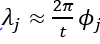 .
.
- Post-Processing
- Sort eigenvalues, compute percentage variance explained, and (optionally) reconstruct eigenvectors classically if full loading is feasible.
Advantages and Disadvantages Compared to the Classical Counterpart #
Advantages #
- Exponential Feature Space Representation – Encoding the covariance matrix as a quantum state embeds dd-dimensional statistics into a 2^n -2^n-dimensional Hilbert space (with n =[log2d]), letting a relatively small qubit register capture correlations that would require massive classical memory.
- Poly-logarithmic Eigenvalue Estimation – Quantum Phase Estimation extracts eigenvalues in O(poly logd) depth under fault-tolerant assumptions, versus classical eigen decomposition, offering asymptotic speed-ups on very large feature sets.
- Spectral‐Gap Amplification – Phase amplitudes scale with the eigenvalue gap, allowing rare-variance directions to be distinguished more cleanly than in floating-point classical PCA, which can suffer from numerical round-off.
- Privacy Preservation Through Quantum States – Because only aggregated density-matrix statistics are uploaded to the quantum back-end, raw records remain on-prem, providing an intrinsic data-obfuscation layer.
- Hybrid Synergy – QPCA slots into classical analytics pipelines: state preparation and result interpretation stay classical, while the expensive diagonalisation step is offloaded to quantum hardware, minimising refactor cost for existing workflows.
Disadvantages #
- State-Preparation Bottleneck – Constructing σ requires O(nd^2) classical time and memory O(d^2), then converts it into quantum amplitudes via O(d) controlled rotations; this overhead can eclipse the quantum speed-up for moderate problem sizes.
- Deep-Circuit Requirements – QPE needs coherent application of U^2k for k ancilla bits; depth grows exponentially with precision, demanding fault-tolerant qubits well beyond today’s NISQ limits.
- Noise-Induced Phase Uncertainty – Gate and read-out errors blur measured phases, collapsing small eigenvalues into sampling noise and requiring heavy error-mitigation or repetition.
- Eigenvector Recovery Still Classical – QPCA returns eigen-values natively; reconstructing eigen-vectors generally needs classical post-processing (or additional tomography), limiting full quantum advantage.
- Parameter-Sensitivity – Poor choices of evolution time t or ancilla precision cause eigen-phase aliasing; tuning these hyperparameters often falls back on classical grid-search.
- Limited Demonstrated Scale – Published demonstrations remain on small (≤ 8-qubit) simulators; no public hardware run has yet beaten classical PCA time-to-solution on real-world data.
Real-World Applications #
| Domain | Quantum Benefit | Example Use-Case | |
| Finance & Risk Analytics | Faster extraction of latent risk factors from large correlation matrices (10⁴–10⁵ assets) | Real-time portfolio Value-at-Risk stress testing | |
| Genomics & Proteomics | Handles 10⁵-dimensional gene-expression vectors where classical PCA is memory-bound | Identifying principal pathways in single-cell RNA-seq data | |
| Climate & Remote Sensing | Compresses multi-spectral satellite imagery with hundreds of bands per pixel | Generating low-rank climate anomaly maps for extreme-weather prediction | |
| Recommender Systems | Quantum speed-up over matrix factorisation for user-item interaction matrices | Producing latent user factors for streaming-media recommendations | |
| Cybersecurity | Detects variance shifts in high-dimensional network-traffic feature sets | Early anomaly detection in zero-trust enterprise networks | |
| Drug Discovery | Reduces millions-dimensional molecular fingerprints to tractable latent spaces | Similarity search for candidate compounds against huge libraries | |
| Industrial IoT | Compresses heterogeneous sensor streams into few principal health indicators | Real-time fault diagnosis in smart-factory equipment | |
| Quantum Chemistry | Uses QPCA as a subroutine to compress quantum states themselves | Identifying dominant electronic configurations in variational eigensolvers |
Overview #
The QPCA_Qniverse implementation delivers a full pipeline for quantum-assisted principal-component extraction inside the Qniverse SDK. Core functionality resides in the QuantumPCA class, while QuantumDimensionalityReducer wraps automated data handling, mixed-type detection (numeric, categorical, mixed), and CSV integration.
Key Components and Features
- Quantum Density-Matrix Builder
Constructs a normalised covariance matrix and rescales it to trace-one for valid state preparation. - Hamiltonian Simulation via expm
Uses SciPy’s matrix exponential to obtain later embedded into a power-of-two unitary. - Flexible Quantum Phase Estimation
User-selectable ancilla count (num_ancilla) and shot count (shots=None for analytic mode). - Automatic Matrix Padding
Pad non-power-of-two matrices with identity blocks, ensuring qubit-register compatibility. - Unified Interface for PCA, MCA, FAMD
Sub-classes (QuantumMCA, QuantumFAMD) share the same quantum core while differing in upstream encoding. - Restricted-Mode Safety
Guards against excessive sample counts (>30) to remain simulation-feasible on commodity hardware. - CSV Autogeneration Helper
In-memory data is saved to a temporary CSV and reloaded, illustrating end-to-end real-world usage.
End-to-End Workflow #
- Initialisation – Instantiate QuantumDimensionalityReducer (optionally set method).
- Data Loading – Pass a 2-D list, NumPy array, or Pandas DataFrame (or an on-disk CSV path).
- Pre-Processing – Automatic type detection, scaling, and one-hot encoding for categorical variables.
- Quantum PCA Execution – Run perform_quantum_pca() with chosen ancilla bits, evolution time, and shots.
- Result Aggregation – Receive density matrix, unitary, measurement histogram, eigenvalues, and metadata in a single dictionary.
- Interpretation – Use QuantumDimensionalityReducer.print_results() for human-friendly insights.
Getting Started in Qniverse #
from qniverse.algorithms import QuantumDimensionalityReducer
# Example: Iris data (first 30 rows for simulation feasibility)
reducer = QuantumDimensionalityReducer()
results = reducer.reduce_from_csv(
data=[
[“sepal_length”,”sepal_width”,”petal_length”,”petal_width”,”species”],
[“5.1”, “3.5”, “1.4” , “0.2”, “setosa”],
# … (up to 30 samples)
],
target_column “species”,
num_ancilla=3,
evolution_time=1.0,
shots=None # analytic mode
)
reducer.print_results(results)
The results dictionary now contains eigenvalues approximating the principal-component variances and the measurement distribution used to obtain them.
Understanding the Parameters #
| Parameter | Purpose |
| num_ancilla | Bits of precision in QPE; more bits ⇒ finer eigen-value resolution (at increased circuit depth). |
| evolution_time (t) | Scales the simulated Hamiltonian; choose tt so that eigen-phases fall within (0,2π)(0, 2\pi). |
| shots | Number of circuit executions. None uses exact probability amplitudes; finite shots introduce sampling noise. |
| restricted_mode | Limits datasets to 30 samples to avoid excessive simulation times on CPUs. |
Hyperparameter Tuning #
Although QPCA lacks a discrete k parameter, users can experimentally adjust:
- Ancilla Count – Trade precision for depth; typical range 3–6 qubits.
- Evolution Time–Scale t to spread eigen-phases; a heuristic is

- Sampling Strategy – Use analytic mode during development; switch to finite shots to model real-device noise.
Evaluation Metrics and Plot History
QPCA returns raw eigenvalues sorted by measurement frequency. Suggested classical follow-up metrics include:
- Explained Variance Ratio –>

- Cumulative Variance –> Determine how many components capture, say, 95 % of total variance.
No plotting is performed automatically; however, the returned eigenvalues can be visualised with conventional Scree plots.
Conclusion #
QuantumPCA offers an insightful bridge between classical covariance analysis and quantum computational primitives. By embedding the covariance structure into a quantum circuit and leveraging QPE, users can explore dimensionality reduction from a quantum vantage point today, while remaining compatible with future fault-tolerant hardware advances. Integrate QPCA into your Qniverse workflows to evaluate quantum readiness for your high-dimensional analytics tasks.