
The Max-Cut Problem #
Given an undirected graph G = (V,E) with vertex set V and edge set E, the Max-Cut problem asks for a partition of V into two disjoint subsets S and V \ S such that the number of edges crossing between the two subsets, i.e., edges (i, j) ∈ E where i ∈ S and j /∈ S is as large as possible.
Formally, the objective is to find a binary assignment x ∈ {0, 1}n (where xi = 0 places vertex i in S and xi = 1 places it in V \ S) that maximises:
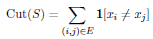
Max-Cut is an NP-hard combinatorial optimisation problem with practical applications in circuit design, statistical physics (the Ising model), and network clustering.
What is the QAOA Max-Cut Algorithm? #
The Quantum Approximate Optimisation Algorithm (QAOA) is a variational hybrid quantum-classical algorithm designed to find approximate solutions to combinatorial optimisation problems. In the context of the Max-Cut problem, the goal is to partition the vertices of a graph G = (V, E) into two sets such that the number of edges between the sets is maximised. Unlike unitary-control protocols, this implementation utilises a classical-quantum feedback loop. The quantum processor prepares a trial state |ψ(γ, β)⟩ parameterised by vectors of angles γ and ⃗β. At the same time, a classical optimizer (e.g., L-BFGS-B, COBYLA, or Differential Evolution) iteratively updates these parameters to minimise the expectation value of the cost Hamiltonian.
Process for QAOA for Max-Cut #
The algorithm prepares the solution state by applying p layers of alternating unitary operators, corresponding to a digitised and variationally optimised adiabatic evolution.
1.Initial State Preparation #
The system starts in a uniform superposition of all possible 2n computational basis states, representing every possible cut configuration. This is the ground state of the mixer Hamiltonian
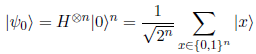
2. The Alternating Unitaries (Layers) #
The algorithm applies p alternating layers, each consisting of two operators:
-
The Cost Layer (HC) #
The cost Hamiltonian HC encodes the Max-Cut objective so that its ground state corresponds to the maximum cut. For each edge (i, j) ∈ E, the operator is defined as:
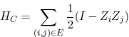
The unitary evolution  is implemented using a CNOT-RZ-CNOT decomposition for each edge(i,j):
1. CX(i, j)
2. RZ(γ, j) (equivalent to 
3. CX(i, j)
-
The Mixer Layer (HB) #
The mixer Hamiltonian HB allows the system to transition between different states in the Hilbert space, ensuring the algorithm can explore the solution landscape and avoid getting stuck in local minima:

The evolution  is implemented by applying RX(2β) gates to every qubit i in the register.
After p such layers, the parameterised trial state is:

3. Energy Estimation and Optimisation #
To find the best cut, we minimise the expectation value of HC over the parameterised state.
This involves three repeated steps:
a) Sampling: The parameterised circuit is executed many times (e.g., 1024 shots). Each execution yields a bitstring x ∈ {0, 1}n representing a candidate cut.
b) Expectation Calculation: The classical computer aggregates the measurement outcomes to estimate the average cut value (energy):

c) Classical Update: The classical optimiser (see Section on optimisers) receives the current energy and adjusts the angles  to find a lower energy on the next iteration. This loop continues until a convergence criterion is met.
Mathematical Foundations: Adiabaticity and Trotterization #
Connection to Quantum Adiabatic Computing (QAC)
In purely continuous Adiabatic Quantum Computing, a system is initialized in the easily preparable ground state of a simple mixing Hamiltonian HB. The system is then subjected to a time-dependent continuous evolution toward the target cost Hamiltonian HC:

The Adiabatic Theorem guarantees that if the total evolution time T is sufficiently long (proportional to the inverse square of the minimum spectral gap), the system will remain in the instantaneous ground state, ultimately culminating in the ground state of HC at t = T, which represents the optimal solution.
Trotterization and Non-Commuting Hamiltonians #
To implement this continuous adiabatic evolution on a gate-based digital quantum computer, we must discretize the time evolution operator  . Because the mixer and cost Hamiltonians do not share eigenstates, they do not commute:
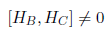
This prevents a clean factorisation of the exponential. The Suzuki-Trotter decomposition provides the remedy for sufficiently small time steps Δt, the evolution can be closely approximated

Applying this over p discrete steps yields the alternating unitary sequence that defines the QAOA circuit.
The Variational Shortcut #
Standard Hamiltonian simulation fixes the step durations to pre-determined values. QAOA departs from this: instead of treating the time steps as constants, it promotes them to variational parameters 
The classical optimiser then minimises  , actively compensating for Trotter errors.
Even at shallow depths (p small), the algorithm does not need to follow the strict adiabatic pathway; it finds an optimised “shortcut” through the Hilbert space, making it a powerful near-term heuristic. As p → ∞, the algorithm theoretically converges to the exact Max-Cut solution.
Final State and Verification #
Upon convergence of the optimizer, the optimal parameters (γ∗, ⃗β∗) are found. The circuit is executed and measured in the computational basis.
- Bitstring Extraction: The most frequent bitstring x ∈ {0,1}n is sampled from the resulting probability distribution.
- Graph Partitioning: Qubits measured as |0⟩ belong to partition S, while qubits measured as |1⟩ belong to partition V\S.
- Cut Value Calculation: The quality of the solution is verified classically by counting edges (i, j) where xi ̸= xj.
Inputs and Outputs #
Inputs #
• Graph type: The user selects one of two graph-generation modes.
– Random graph: the implementation generates a random graph with the specified number of nodes. Edge probability can be controlled via implementation parameters.
– Custom graph: the user manually specifies the graph structure by providing the number of nodes together with an explicit edge list in the format:
[[a1, b1], [a2, b2], [a3, b3], . . .]
where each pair ak, bk denotes an edge between vertices ak and bk.
Number of nodes (n): An integer in the range [3, 28]. The upper bound of 28 reflects the memory constraints of classical state-vector simulation at this depth.
Number of QAOA layers (p): A positive integer controlling the circuit depth. Higher values of p generally improve approximation quality at the cost of a larger circuit and a higher-dimensional optimisation landscape.
Optimiser: One of the nine classical optimisers listed in the following section.
Outputs #
Best bitstring: The most frequently sampled measurement outcome encoding the proposed partition (e.g. 0110), where each bit corresponds to the group assignment of the respective vertex.
• Cut value: The number of edges crossing the proposed partition, computed classically from the bitstring for verification (e.g., a cut value of 4 for a 4-node complete graph).
Energy: The minimised expectation value returned by the optimiser. This is a negative quantity whose magnitude reflects the quality of the solution; a lower (more negative) value indicates a better cut.
• Execution time: The wall-clock time (in seconds) taken by the optimisation loop to converge.
• Graph structure: The full description of the problem instance, i.e., the node list, edge list, and the 2D layout positions of each vertex, is returned alongside the solution for visualisation purposes.
• Partition colouring: Each vertex is assigned a group label (0 or 1) corresponding to the two sides of the cut, together with a display colour, enabling direct visual rendering of the Max-Cut solution on the graph.
Key Features of this Implementation #
• Optimizer Versatility: Supports 9 distinct optimization strategies, allowing for the empirical study of parameter landscapes using gradient-based (Adam), derivative-free (COBYLA), and global stochastic methods (Differential Evolution).
• Layered Scalability: Adjustable depth p allows for a trade-off between circuit complexity, Trotter error relaxation, and approximation accuracy. As p → ∞, the algorithm theoretically converges to the exact Max-Cut.
• Hardware Agnostic: Compatible with both CPU (lightning.qubit) and GPU-accelerated (lightning.gpu) simulators, enabling the scaling of simulated nodal networks up to memory limits.
Classical Optimisers #
Nine classical optimisation strategies are supported, spanning gradient-based, derivative-free,
and global stochastic methods.
• L-BFGS-B (Limited-memory Broyden–Fletcher–Goldfarb–Shanno with Bound constraints):
A quasi-Newton gradient-based method that approximates the inverse Hessian using a limited history of gradient evaluations. Efficient and fast when gradients can be estimated accurately, but may settle in local minima.
• COBYLA (Constrained Optimisation BY Linear Approximations): A derivative-free method that builds successive linear approximations to the objective. Well-suited to noisy quantum landscapes where gradient computation is expensive.
• Nelder–Mead: A simplex-based, derivative-free downhill search. Robust to noise and easy to tune; convergence can be slow in high-dimensional parameter spaces.
• Powell: A derivative-free method that performs successive line minimisations along conjugate directions. Generally faster than Nelder–Mead but still gradient-free.
• SLSQP (Sequential Least-Squares Quadratic Programming): A gradient-based method that solves a sequence of quadratic sub-problems. Accurate and fast when the energy landscape is smooth.
• Adam: A first-order stochastic gradient method with adaptive per-parameter learning rates. Handles noisy gradient estimates well; widely used in machine learning contexts.
• Adagrad (Adaptive Gradient Algorithm): Accumulates squared gradients to scale the learning rate for each parameter individually. Effective when some parameters exhibit sparse updates.
• Differential Evolution (DE): A global, population-based stochastic search that evolves a set of candidate parameter vectors through mutation and crossover. Less likely to be trapped in local minima, but requires more function evaluations.
• Hybrid Differential Evolution: Combines the global exploration of Differential Evolution with a gradient-based local refinement step (e.g. L-BFGS-B) to polish the best candidate found by DE. Balances broad exploration with high-precision local convergence.
Advantages and Disadvantages #
Advantages #
• Near-term hardware compatibility: QAOA circuits are relatively shallow (depth scales as O(p|E|)) and consist entirely of single- and two-qubit gates, making the algorithm a strong candidate for current and near-term noisy intermediate-scale quantum (NISQ) devices.
• Theoretical convergence guarantee: As the number of layers p increases, the algorithm is guaranteed to converge to the exact Max-Cut solution, providing a rigorous quality ladder.
• Optimiser flexibility: Support for nine distinct optimisers allows empirical study of the parameter landscape and the selection of the most effective strategy for a given graph instance or noise level.
• Scalable simulation: The CPU-based lightning qubit simulator enables state-vector simulation up to 28 qubits within available memory, covering a non-trivial range of problem sizes.
• Hybrid exploitation: Hybrid Differential Evolution and other combined strategies can leverage the complementary strengths of global and local search, reducing the risk of premature convergence.
• Problem generality: The QAOA framework extends beyond Max-Cut to a wide class of quadratic unconstrained binary optimisation (QUBO) problems with minimal modification.
Disadvantages #
• Classical simulation overhead: Exact state-vector simulation scales exponentially in the number of qubits (2n complex amplitudes), limiting classical emulation to n ≤ 28 nodes in this implementation.
• Barren plateaus: For large n or deep circuits, the gradient of the cost function with respect to the variational parameters can become exponentially small, a phenomenon known as barren plateaus, thus making gradient-based optimisers ineffective without mitigation strategies.
• Local minima sensitivity: Derivative-free and gradient-based local optimisers (COBYLA, Nelder–Mead, L-BFGS-B) are susceptible to convergence at sub-optimal local minima, particularly for dense or large graphs.
• High shot count: Accurate expectation-value estimation requires many circuit executions (shots), increasing the total runtime, especially as the number of edges and parameters grows.
• No optimality certificate: QAOA provides an approximate solution whose quality depends on p, the optimiser, and the initialisation of parameters. There is in general, no guarantee that the returned cut is optimal for a fixed p.
• Parameter initialisation sensitivity: The quality of the final solution can be sensitive to the initial values of ⃗γ and ⃗β, and poor initialisations may require many restarts.
• Trotter error at low depth: At small p, the Trotterisation of the adiabatic path introduces non-negligible approximation error, which the variational optimiser can partially but not fully compensate.