
What is Trotterization? #
In quantum mechanics, the way a system changes over time is governed by its Hamiltonian H. If you know the starting state ψ(0)⟩, then the exact state at time T is given by:
|ψ(T )⟩ = e−iHT |ψ(0)⟩ .
The challenge is that in most real problems, H isn’t a single simple operator. It’s a sum of several pieces,
![]()
where each Pj is a Pauli string (like X ⊗ Y ⊗ Z) and αj is a real coefficient. If all these terms commuted with each other, life would be easy; we could exponentiate them all at once. But they don’t. And that’s where Trotterization comes in.
Presenting here with a short video tour of how the Time-Evolution of a Quantum System using the Trotterization Algorithm works in Qniverse
The core idea
Instead of trying to apply e^−iHT directly, we slice the total evolution time T into N tiny steps of size ∆t = T /N. At each step, we apply short evolutions from the individual Hamiltonian terms sequentially. When we repeat this process N times, the resulting product of small operations closely approximates the true e^−iHT.
The necessary formulas
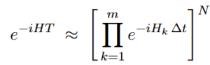
If ![]() , with each Hk being a part of the Hamiltonian, we can implement:
, with each Hk being a part of the Hamiltonian, we can implement:
• First-order (Lie–Trotter) formula:
• Second-order (Strang splitting):
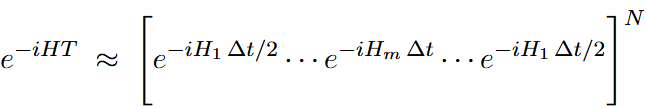
The second-order version generally gives better accuracy for the same number of steps, because it cancels out more of the error terms.
How accurate is this? #
The error comes from the fact that the Hk terms don’t commute. Using the Baker–Campbell– Hausdorff (BCH) formula, we can see that,
• With first-order Trotterization, the global error scales as O(T ∆t).
• With second-order, it improves to O(T ∆t2).
Therefore, reducing ∆t (i.e., using more steps, N ) or switching to higher-order formulas decreases the error. Fourth-order and beyond exist, but they require more gates per step—so on current hardware, second-order is often the sweet spot.
Why does this matter? #
Quantum hardware doesn’t let you apply e−iHT as a single gate. It only gives you basic one- and two-qubit operations. Trotterization is the bridge: it translates a Hamiltonian into an actual circuit made of gates.
It also gives you control. By tuning the number of steps N and the order of the formula, you can balance accuracy against circuit depth. That makes Trotterization the practical backbone of simulating quantum dynamics on today’s machines and the benchmark for more advanced Hamiltonian-simulation methods.
Most interesting Hamiltonians are sums of non-commuting terms, so we cannot apply e−iHT in one shot. Trotterization breaks the problem into gates we can implement and gives us clean dials (order and N ) to trade depth for accuracy:
εglobal = O(T ∆tp), p = 1, 2, . . .
In practice, start with the second order and a modest N, check fidelity, and adjust. That’s the core loop you’ll follow in Qniverse: fast, empirical, and effective.
How is Trotterization done in Qniverse? #
What you prepare
• Hamiltonian as a sum of Pauli strings with real coefficients, e.g., 0.5 ˆX ⊗ ˆZ ⊗ ˆI − 1.2 ˆY ⊗ˆY ⊗ ˆX + ˆZ ⊗ ˆY ⊗ ˆX.
• Initial state (basis bitstring like |000⟩ or a simple superposition); normalization is handled by the tool.
• Total time T, order (1 or 2 to start), and number of Trotter steps N (sets ∆t =T /N ).
How is this implemented in Qniverse? #
1. Open the Suzuki–Trotter card in the algorithm catalog and click Load Circuit to open the parameter dialog.
2. Fill the fields: Hamiltonian, initial state, order, steps N, and total time T.
3. Click Load Graph to preview a live plot of fidelity vs. steps N for the chosen order. Use this to choose the smallest N that brings fidelity near 1 while keeping circuits shallow.
4. Click Load /Run to build and execute the circuit on the selected backend (simulator or available hardware).
5. Read the results: the result pane reports (i) the fidelity F ∈ [0, 1] between exact and Trotterized evolution and (ii) the final state |ψ(T )⟩ in Dirac notation. If F is lower than you want, increase N or move from first to second order and re-run.
What actually happens under the UI (intuitive math)? #
Each short exponential in a slice has the form e^−iαj Pj ∆t, where Pj is a Pauli string. Qniverse implements it via:
![]()
where Rj rotates the qubits so that Pj becomes Z⊗r (a diagonal operator), applies a phase rotation about Z (using standard CNOT “pack/unpack” patterns), and then rotates back.
Repeating the ordered product of these per-term exponentials N times yields the full Trotterized circuit for time T.
Fidelity (what the graph shows). If |ψexact(T )⟩ = e−iHT |ψ(0)⟩ and |ψTrot(T )⟩ is the Trotterized state, the overlap
![]()
quantifies accuracy. On the preview graph, watch how F improves with N and with the chosen order (1 vs. 2). For fixed T, halving ∆t (doubling N ) reduces first-order global error roughly by ×2; second order drops faster.
Worked 3-qubit example #
Consider the 3-qubit Hamiltonian
H = 0.2 (X ⊗Y ⊗Z) + 0.5 (Y ⊗Y ⊗X) + 0.4 (Y ⊗Y ⊗Y ) + 0.8 (Y ⊗Z ⊗Y).
Goal: simulate U (t) = e−iHt for t = 0.01 with initial state |ψ(0)⟩ = |000⟩.
Pick parameters and run. Choose the first order with N = 25 steps, so ∆t = t/N = 0.0004. In the dialog: enter H term by term, set t, order = 1, steps N = 25, and |000⟩ as the initial state. Load the graph to confirm fidelity is already high, then run. You should see a fidelity close to 0.9998 for these settings.
What to try next. Switch to second order with a smaller N and compare the fidelity curve; you’ll typically match or exceed accuracy with fewer steps. If you increase t, expect to raise N (or the order) to keep accuracy similar.
Potential Uses and Applications #
• Quantum chemistry and materials: real-time dynamics, short-time response, and state preparation for small molecules and model Hamiltonians.
• Condensed matter/lattice models: non-commuting spin models, quenches, and transport in toy models (e.g., Schwinger model discretizations).
• Benchmarking and education: a clear, controllable baseline for teaching Hamiltonian simulation and for validating more advanced methods.
• Scientific pipelines: a practical front end to explore error-depth trade-offs before moving to higher-order formulas or alternative simulators.